Rethinking probabilities

This post is based on this article.

Does it even make sense to discuss about adding two probabilities?

Probabilities definitely look like vectors: they are arrays of numbers. For example, it could make sense that a coin toss would be described by an array with two numbers, something like $(0.5, 0.5)$.

However, it is not obvious how they would inherit any kind of vector space structure (if you need a reminder on vector spaces, Wikipedia is your friend). Here, by vector space, we intuitively mean a space where the operations of

1. Adding two vectors, and
2. Multiplying a vector by a scalar

are well-defined.

Clearly, element-wise addition doesn’t work for probability vectors: adding the coin toss vector above to itself would yield something like $(0.5+0.5, 0.5+0.5) = (1,1)$, which cannot be a probability since its components do not sum up to 1.

Element-wise multiplication by a scalar suffers from the same issue.

Going to $\mathbb{R}^n$ and back again

Let $\Delta_{K}$ be the $K+1$-dimensional probability simplex, which is the natural place for probabilities to live in:

$$\Delta_K := \left\{ p \in [0,1]^{K+1}: \sum_{k=1}^{K+1} p_k = 1 \right\}$$

Define the logit function as the map $\phi: \Delta_K \to \mathbb R^{K}$ such that, if $p_i$ is the $i$-th component of $p$, then

$$\boxed{\phi(p)_i = \log \frac{p_i}{p_{K+1}}}\quad\text{(logit function)}$$

where the last component $p_{K+1}$ is equal to $1 - \sum_{k=1}^K p_k$.

This function, for the case of binary distributions, is the common logit function used in logistic regression, $\log (p/(1-p))$. This is a natural multidimensional extension.*

It is easy to show that the inverse logit function will be given by

$$\phi^{-1}(x)_i = \begin{cases} \displaystyle \frac{e^{x_i}}{Z} & \text{ if } i \in \{1,\cdots,K\}\\ \displaystyle \frac{1}{Z} & \text{ if } i = K+1 \end{cases}$$

where the normalization is

$$Z = 1 + \sum_{k=1}^K e^{x_k}$$

In order for us to endow $\Delta_K$ with a vector space structure, we will define all vector space operations by

• first going from $\Delta_K$ to $\mathbb R^K$ via the logit function…
• then doing linear algebra in $\mathbb R^K$…
• and finally mapping back to $\Delta_K$ via the inverse logit function.

To make notation a bit clearer, we will start writing probability vectors by borrowing the bra-ket notation from quantum mechanics. This is just a fancy way to tell vectors in $\Delta_K$ apart from their components in $\mathbb R^{K+1}$, which have no vector structure.

Let us define the sum of two points in the simplex as

$$\boxed{|p\rangle + |q\rangle := \phi^{-1}(\phi(p) + \phi(q))}$$

and the multiplication by scalar as

$$\boxed{\alpha |p\rangle := \phi^{-1}(\alpha\, \phi(p))}$$

It is easy to show that these two yield

$$(|p\rangle+|q\rangle)_i = \frac{1}{ \sum_{k=1}^{K+1} p_k q_k} p_i q_i$$ $$(\alpha | p\rangle)_i = \frac{1}{\sum_{k=1}^{K+1} p_k^\alpha} p_i^\alpha$$

Some important results:

1. The null vector in $\Delta_K$ is the one relative to the uniform distribution:

$$|0\rangle_i= \frac{1}{K+1}.$$

Indeed, it is easy to show that $\vert p\rangle + \vert 0\rangle = \vert p\rangle$ for any $p$.

2. The additive inverse, which we call $\vert - p\rangle$, is exactly $(-1)\vert p\rangle$:

$$|- p\rangle_i = (-1 |p\rangle)_i = \frac{1/p_i}{\sum_{k=1}^{K+1} 1/p_k}$$

With these operations, $(\Delta_K, +, \cdot)$ is a real vector space! We can, by extention, calculate linear combinations: it is straighforward to show that the components of $\alpha \vert p \rangle + \beta \vert q \rangle$ are given by

$$(\alpha \vert p \rangle + \beta \vert q \rangle)_i = \frac{\displaystyle1/(p_i^\alpha q_i^\beta)}{\displaystyle \prod_j 1/(p_j^\alpha q_j^\beta)}$$

Implementing this in Python

Python allows us to overload the + operation. Below, we implement a class Prob which takes the components of a probability vector and transforms it into a proper vector space element.

from __future__ import annotations

class Prob:
    
    def __init__(self, 
                coords: np.array):
        
        self.p = np.array(coords)
        self.dimension = self.p.shape[0]
    
    def __add__(self, q: Prob):
        assert self.dimension == q.dimension, "Probability vectors must have the same dimension"
        summ = self.p * q.p
        summ /= summ.sum()
        
        return Prob(coords=summ)
    
    def __sub__(self, q: Prob):
        return self.__add__(q.scalar(-1))
    
    def __mul__(self, a: float):
        
        return self.scalar(a)
    
    def scalar(self, a: float):
        
        coords = (self.p)**a
        coords /= coords.sum()
        return Prob(coords=coords)
    
    def __repr__(self):
        return "("+ ", ".join([str(round(p,4)) for p in self.p]) + ")"
    
    @classmethod
    def zero(clf, dimension: int):
        return Prob(1/dimension*np.ones((dimension)))

Let us run some tests. First, we start from two vectors and the zero vector:

p = Prob([0.3, 0.3, 0.4])
q = Prob([0.2, 0.1, 0.7])

# see if zero is properly implemented
zero = Prob.zero(dimension=3)
zero

# >> (0.3333, 0.3333, 0.3333)

Try summing vector $\vert p\rangle$ with $\vert 0\rangle$; nothing should change:

p+zero # zero doesn't do anything
# >> (0.3, 0.3, 0.4)

We can also check the components of $\vert-p\rangle$; notice that Python requires us to write this as p * (-1) instead of -1 * p:

p_bar = p * (-1) # how does the additive inverse look like?
p_bar
# >> (0.3636, 0.3636, 0.2727)

By consistency, $\vert p\rangle + \vert -p\rangle$ should equal $\vert 0\rangle$:

p+p_bar # should give the zero vector
# >> (0.3333, 0.3333, 0.3333)

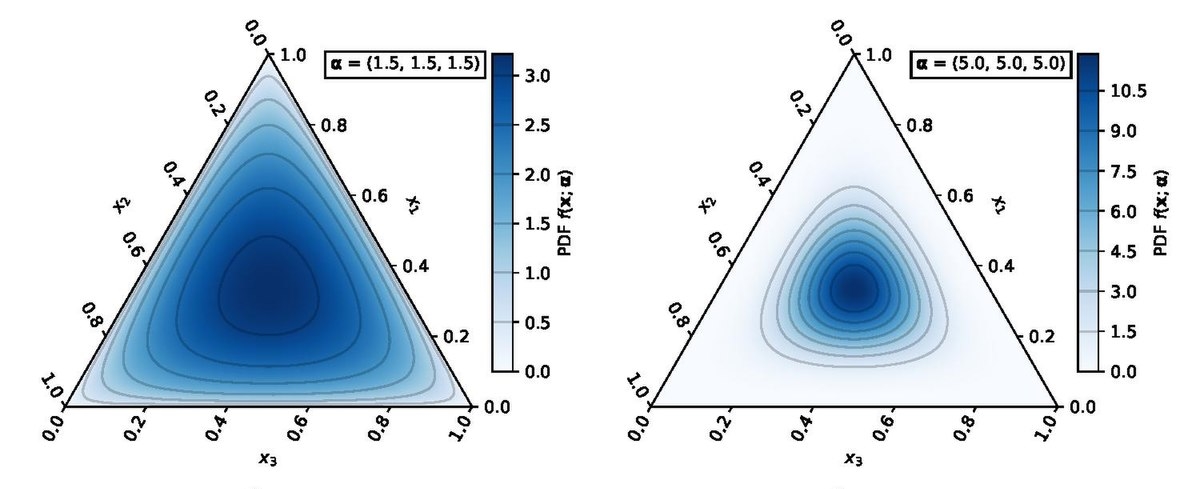
We can also make some plots. Since our vectors live on the 2-simplex $\Delta_2$, which is basically a triangle (see the image on the top of this post), visualization is pretty straightforward.

Below, we make a simple experiment: we take a vector to Euclidean space, rotate it by some angle, and map it back via the inverse logit function.

def plot_simplex(y_true, y_probs, ax=None):
    
    simplex_coords = lambda x, y, z:  ((-x+y)/np.sqrt(2), (-x-y+2*z+1)/np.sqrt(6))
    xs, ys = simplex_coords(y_probs[:,0], y_probs[:,1], y_probs[:,2])
    if ax is None:
        plt.plot(xs, ys, c=y_true, alpha=0.5, marker='.')
        plt.show()
    else:
        ax.plot(xs, ys, c=y_true, alpha=0.5, marker='.')

def logit2(p):
    p1, p2, p3 = p[0], p[1], p[2]
    
    return np.array([np.log(p1/p3), np.log(p2/p3)])

def inv_logit2(x):
    xx = np.append(x,0)
    Z = 1 + np.exp(x).sum()
    return 1/Z * np.exp(xx)

p = np.array([0.3, 0.1, 0.6])
assert np.all(inv_logit2(logit2(p)) == p)

def rot(theta):
	'''2D vector rotation by angle theta'''
    c, s = np.cos(theta), np.sin(theta)
    return np.array([[c, s],[-s,c]])

fig, ax = plt.subplots()

for p in [
    np.array([0.9, 0.05, 0.05]),
    np.array([0.99, 0.005, 0.005]),
    np.array([0.33, 0.33, 0.34]),
    np.array([0.6, 0.2, 0.2]),
]: 
    rotated_x = [rot(theta) @ logit2(p) for theta in np.arange(0, 6.28, 0.01)]
    rotate_p = [inv_logit2(xx) for xx in rotated_x]
    plot_simplex(None, np.array(rotate_p), ax)
    
ax.plot([-1/np.sqrt(2), 0], [0, np.sqrt(3/2)], color='gray')
ax.plot([0, 1/np.sqrt(2) ], [np.sqrt(3/2), 0], color='gray')
ax.plot([-1/np.sqrt(2), 1/np.sqrt(2)], [0, 0], color='gray')
plt.show()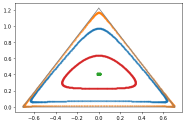

Notice how rotating and mapping back makes our circles bend, in order for them to stay inside the probability simplex.

Is that it?

The space of probabilities is an important and rather misunderstood one. I have previously studied distance functions in these spaces (post to be written soon) as well as clustering inside the probability simplex, but the future outlook is still open.