Context
This was originally written as a quick intro to partial AUCs, aimed at giving my team at the DataLab some insights into cost-based classification.
Below, we consider the standard binary classification problem.
Assume we pay a cost in case we classify a point of the positive class as a negative, and, similarly, pay a cost in case of a false positive.
With no loss of generality, we assume these costs are normalized and sum to one:
(if they are not, we can normalize via and similarly for ).
For a given classification threshold , what is the total misclassification cost? Assume we have total points, out of which real positives and real negatives, where
Then the total false positives and false negatives is, written in terms of the coordinates of the ROC curve,
multiplying these by the specific costs we get
Equation is the general cost at any given .
Now, what is our baseline of comparison? That would be the random model where we set
It is easy to see that this model leads to regardless of the threshold, hence a cost of
Thus, a good model needs to give a cost lower than random guessing, ie. , ie.
or
We then arrive at the following criterion:
Cost based partial AUC
- Let denote the prevalence of the positive class
- Let denote the cost of a false negative
Then, the region in the ROC plane bounded below by
and bounded above by the ROC curve defines the “useful” area from a cost perspective,
Examples and implementation
A “clean” implementation follows after these first examples.
(a) Balanced case
X, y = make_classification(n_classes=2,
                           n_samples=3000,
                           random_state=2,
                           n_features=10,
                           n_informative=10,
                           weights=(0.5,),
                           n_redundant=0,
                           n_repeated=0)

model = LogisticRegression()
model.fit(X, y)

y_probs = model.predict_proba(X)[:,1]

fpr, tpr, thresh = roc_curve(y, y_probs)

pi = y.mean()

for cost_fn in [0.3, 0.5, 0.8]:
    cost_fp = 1 - cost_fn
    rho = cost_fn

    tpr_base = 1 - (1-pi)/rho + (1-rho)/rho * (1-pi)/pi * fpr
    pauc = auc(fpr, np.maximum(tpr-np.maximum(0,tpr_base),0))

    # maximum value
    aux = np.clip(tpr_base,0,1)
    max_pauc = 1 - auc(fpr, aux)


    plt.plot(fpr, tpr_base,
             label=f'FN cost: {cost_fn}\n(pAUC: {round(pauc,2)}\nMaxpAUC: {round(max_pauc,2)})',
             linestyle='--')


plt.plot(fpr, tpr)
plt.xlim(0,1)
plt.ylim(0,1)
plt.legend()
plt.show()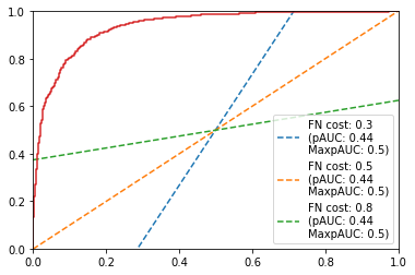
Notice that, in this balanced case, the fact that we are using a cost-based partial AUC doesn’t change much: all AUCs are basically equal.
(b) Imbalanced case
X, y = make_classification(n_classes=2,
                           n_samples=3000,
                           random_state=2,
                           n_features=10,
                           n_informative=10,
                           weights=(0.8,),
                           n_redundant=0,
                           n_repeated=0)

model = LogisticRegression()
model.fit(X, y)

y_probs = model.predict_proba(X)[:,1]

fpr, tpr, thresh = roc_curve(y, y_probs)

pi = y.mean()

for cost_fn in [0.3, 0.5, 0.8]:
    cost_fp = 1 - cost_fn
    rho = cost_fn

    tpr_base = 1 - (1-pi)/rho + (1-rho)/rho * (1-pi)/pi * fpr
    pauc = auc(fpr, np.maximum(tpr-np.maximum(0,tpr_base),0))

    # maximum value
    aux = np.clip(tpr_base,0,1)
    max_pauc = 1 - auc(fpr, aux)


    plt.plot(fpr, tpr_base,
             label=f'FN cost: {cost_fn}\n(pAUC: {round(pauc,2)}\nMaxpAUC: {round(max_pauc,2)})',
             linestyle='--')


plt.plot(fpr, tpr)
plt.xlim(0,1)
plt.ylim(0,1)
plt.legend()
plt.show()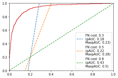
Notice how adding imbalance changes the game significantly.
Functional implementation
Below, as a reference, we leave a function to calculate these metrics following a syntax close to the scikit-learn one.
def cost_based_roc_auc(y_true, y_probs,
                       cost_fn=None,
                       cost_fp=None,
                       return_curves=False):
    from sklearn.metrics import roc_curve, auc

    fpr, tpr, thresh = roc_curve(y_true, y_probs)

    is_fn_none = cost_fn is None
    is_fp_none = cost_fp is None

    assert not all([is_fn_none, is_fp_none]), "At least one out of cost_fn and cost_fp needs to be not None"

    if is_fn_none:
        assert 0 <= cost_fp <= 1
        cost_fn = 1 - cost_fp
    else:
        assert 0 <= cost_fn <= 1

    pi = y_true.mean()

    rho = cost_fn

    tpr_base = 1 - (1-pi)/rho + (1-rho)/rho * (1-pi)/pi * fpr
    pauc = auc(fpr, np.maximum(tpr-np.maximum(0,tpr_base),0))

    # maximum value
    max_pauc = auc(fpr, 1 - np.clip(tpr_base,0,1))

    if not return_curves:
        return pauc, max_pauc
    else:
        return pauc, max_pauc, fpr, tpr, tpr_base
for cost_fn in [0.1, 0.3, 0.5, 0.8, 0.9]:
pauc, pauc_max = cost_based_roc_auc(y, y_probs, cost_fn=cost_fn)
print(f"Cost FN {cost_fn}: {round(pauc/pauc_max,2)} %")
# >> Cost FN 0.1: 0.75 %
# >> Cost FN 0.3: 0.76 %
# >> Cost FN 0.5: 0.78 %
# >> Cost FN 0.8: 0.86 %
# >> Cost FN 0.9: 0.9 %