Our task

I am not a game designer; I have never used any engines such as Unity, nor have I done any 3D modeling before. Buuuuut…

I really like simulating physical systems. In my opinion, most Physics undergraduate curricula lack one thing in common: more emphasis on numerical simulations, be it solving the relevant differential equations (e.g. electromagnetic waves, quantum systems) or simulating complex systems, like gravitational N-body simulations.

On top of that, I often like to reinvent the wheel as a learning mechanism. Someone said:

When you reinvent the wheel, you end up learning a great deal about why wheels are round.

Instead of starting from a textbook, I often prefer the (10x more time-consuming) approach of thinking hard about a problem and trying to solve it myself. Once I get tired of this long-winded endeavor and finally decide to check real references, there is this warm feeling of reading about something I had already rediscovered or, at least, contemplated.

So, on that note, I will build a formalism for running simulations of particles contained inside a volume of any shape.

By the way: most methods here will be expensive, as in $O(n^2)$ or $O(n^3)$ in the number of particles. Maybe it can be optimized in the future, for instance by being more careful about partioning space.

Formalism of things hitting walls

The most natural mathematical framework for us is to consider physical space as being $\mathbf R^n$ (where $n$ can be 2 or 3) and time to be a discretized set of time-steps $\{t_1=0,t_2,\ldots, t_n=T\}$.

Now, we want to consider a substance moving around inside a volume. The conceptually simplest description we can use is that of particles that don’t interact among themselves. We know from ideal gas theory that, despite this simplified assumption, we can retrieve many properties of realistic systems from this description.

And this is indeed the endgame, but I will leave this for some future post.

With that being said, we want our particles to be able to interact with the walls of whatever compartment they are in. So it makes sense to consider a formalism where we can easily define a volume and its walls.

Geometry: domains and walls

We define the domain where our gas lives as the locus

$$\boxed{\Omega \equiv \{x \in\mathbf R^n:\omega(x) >0\}}$$

where $\omega: \mathbf R^n \to \mathbf R$ is some real-valued function.

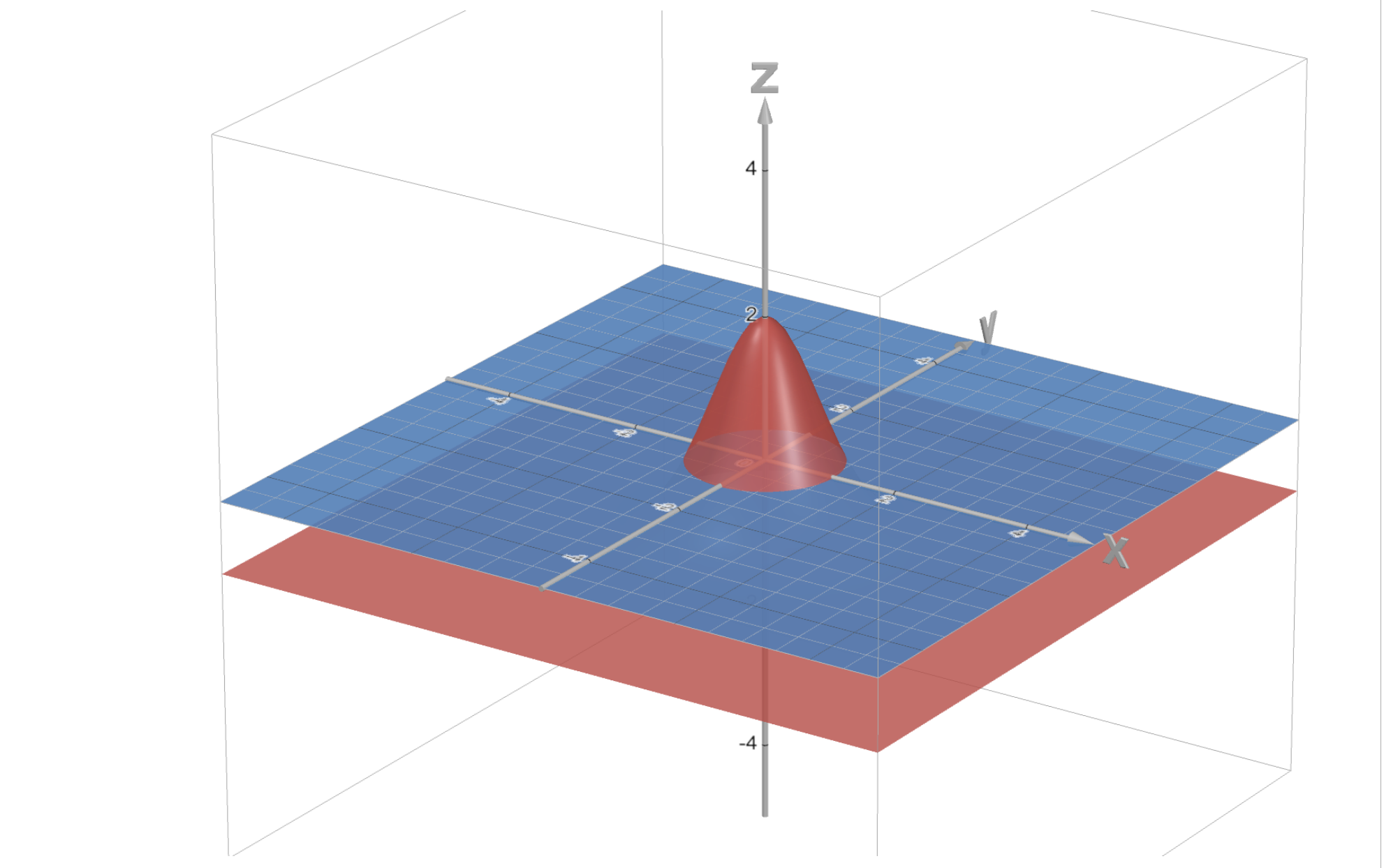
Example: one could choose $\omega(x,y) = 3\exp(-x^2-y^2) - 1$. This function is positive inside the circle of radius $\sqrt{\log 3}$, zero on the circle, and negative outside, hence our particles would be living inside the circle.

What do we require of $\omega$? It makes sense for it to be continuous; we keep other hypotheses regarding smoothness on hold for now.

Now let us consider a single particle. Its position at any time $t_i$ is given by a vector $x(t_i)$, which evolves according to Newton’s second law. Numerically, we know how to do this via various algorithms, such as the Euler method, leapfrog integration or Runge-Kutta methods.

The leapfrog method is known for being much better than the others at conserving energy, hence it is the one we will use.

We assume that there exists an algorithm $\mathrm{evolution}()$ which takes an initial position, an initial velocity, and a timestep, and returns the next position and velocities:

$$\boxed{x_{t+\Delta t}, v_{t+\Delta t} = \mathrm{evolution}(x_t, v_t, \Delta t).}$$

This immediately means we do not consider interactions among the particles; otherwise the right-hand side would containg the whole list of positions and velocities for all particles.

But collisions against walls are not 100% included in this formalism: they are, effectively, an instantaneous infinite force applied to the particle. Hence we need to come up with a procedure to simulate collisions.

Define the wall as the boundary

$$\partial \Omega=\{x\in\mathbf R^n:\omega(x)=0\};$$

I am pretty confident that requiring $\partial \Omega$ to be a regular surface should be enough; numerically, we can accept a few (ie. finite number of) points where the normal vector is not well-defined, since there is zero probability a particle will collide with them.

Then, on what follows, I assume

$$\hat n(x) = \frac{\nabla \omega(x)}{|\nabla \omega(x)|},\quad x \in \partial \Omega$$

is a well-defined, inward- pointing normal vector.

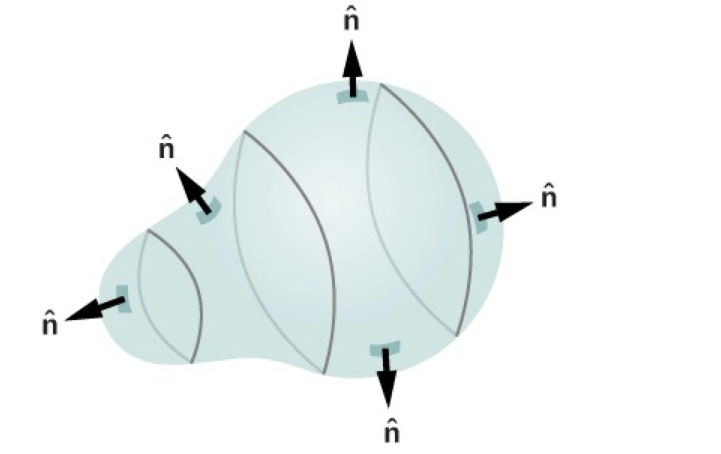
Usually, normal vectors are defined outward-pointing — see the figure below for an example (source). We choose inward since we care about the geometry inside the domain, which depends on the inward normal. You can equivalently define $\hat n$ as the outward-pointing normal vector and formally substitute $\hat n \to -\hat n$ in all subsequent formulas.

Collision detection

Since time is discretized, we can consider a particle’s trajectory $x(t)$ as being sampled over time steps: $x(t_0), x(t_1),\ldots, x(t_n)$. If we observe a situation where

$$x(t_i) \in \Omega\quad \text{ but }\quad x(t_{i+1})\notin \Omega \qquad (\text{i.e.}\quad \omega(x(t_i)) > 0,\quad \omega(x(t_{i+1}))\leq 0)$$

then we can be sure there should have been a collision against the wall at some instant in $]t_{i}, t_{i+1}]$; we then need to artificially change $x(t_{i+1})$ so that it accounts for collision effects.

Can we find out when the collision happened? For simplicity call $x_i \equiv x(t_i)$. Let us assume that the trajectory between $x_i$ and $x_{i+1}$ is approximately linear, so that it can be parameterized by $\lambda \in [0,1]$ as $x_i + \lambda (x_{i+1}-x_i)$. By continuity of $\omega$, there exists $\lambda_\star$ such that

$$\boxed{\omega(x_i+\lambda_\star(x_{i+1}-x_i))=0.}$$

Assuming $\vert \lambda_\star (x_{i+1} - x_i)\vert$ to be small, we can Taylor expand to first order and solve for $\lambda_\star$:

$$\lambda_\star \approx - \frac{\omega(x_i)}{(x_{i+1} - x_i)\cdot \nabla \omega(x_i)}.$$

Notice that calculating this quantity is slightly expensive — it requires us to compute the gradient at $x_i$.

There is an even more precise way: we could expand both around $x_i$ and $x_{i+1}$ and combine the results.

So now we know how far along the segment between the two points one should find the collision point, namely,

$$x_*=x_i+\lambda_\star (x_{i+1}-x_i).$$

Shifting positions and velocities

By geometry (see discussion below), we can now find that the new position for the reflected particle is

$$\boxed{x_{i+1}' = x_{i+1}-2(1-\lambda_\star)[(x_{i+1}-x_i)\cdot \hat n_*] \hat n_\star}$$

where $\hat n_\star \equiv \hat n(x_\star)$.

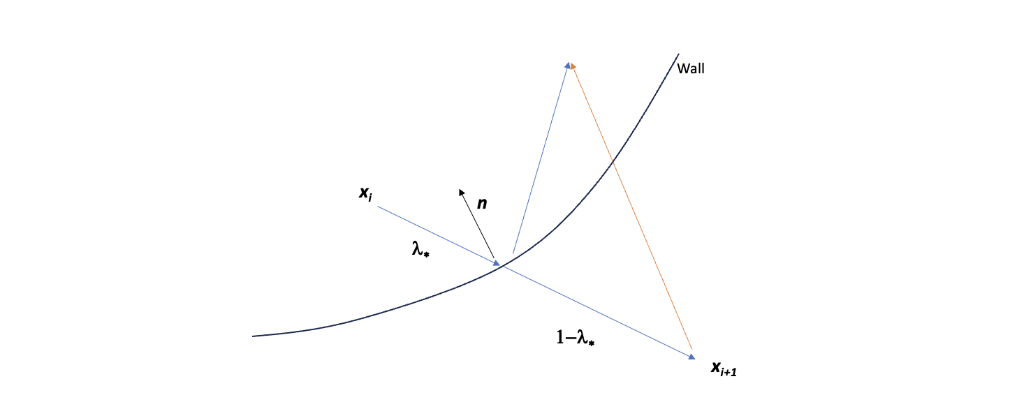
The proof is as follows: the vector pointing from $x_i$ to $x_{i+1}$ is their difference $x_{i+1}-x_i$. Its projection along the surface normal $\hat{n}_\star$ is

$$[(x_{i+1}-x_i)\cdot \hat{n}_\star]\hat{n}_\star.$$

From $x_{i+1}$, how much do we need to “walk along” the projection? Since it takes “time” $\lambda_\star$ to go from $x_i$ to the wall ($x_\star$), we are left with an amount of $1-\lambda_\star$ of time to go up; we need a factor of 2 to walk the same amount from $x_{i+1}$. Hence,

$$x_{i+1}'= x_{i+1} - 2(1-\lambda_\star)[(x_{i+1}-x_i)\cdot \hat n_\star]\hat n_\star$$

as we wanted to prove.

What happens to the velocity? Consider the velocity vector $v_-$ right before collision. The component parallel to the wall normal, ie.

$$v_\parallel \equiv v_- \cdot \hat{n}_\star$$

is inverted after the elastic collision; the perpendicular component

$$v_\perp \equiv v - (v_{-} \cdot \hat{n}_\star)\hat{n}_\star$$

is kept equal. Hence, a shock against that wall corresponds to the following map:

$$v_- \mapsto v_+ = v_- - 2( v_-\cdot \hat n_\star) \hat n_\star$$

However, what is the best approximation we have for $v_-$? Given $v_i \equiv v(t_i)$, we know that a time of $\lambda_\star(t_{i+1} - t_i)$ is elapsed since $t_i$ and the hypothetical collision instant; hence, the velocity right before collision is

$$\underline{\;\;} , v_- = \mathrm{evolution}(x_0 = x(t_i),\; v_0 = v(t_i),\; \Delta t = \lambda_* (t_{i+1} - t_i))$$

This step is very expensive — it requires another computation of evolution. For small time steps, it is likely that just using $v_- \approx v(t_i)$ would be sufficient.

Hence, we have all the ingredients for an algorithm. We first tentatively evolve all particles to their next position; then, if any fall out of the domain, we fix their position and velocity via the procedures above.

INPUTS:

• Function $\omega(x)$ and its gradient $\nabla \omega(x)$ - ideally $\omega$ must be cheap to evaluate and its gradient must be pre-calculated analytically
• $N$ particles with mass $m$ and initial positions / velocities $x^{(i)}_0, v^{(i)}_0$ (here $i \in \{1,\ldots, N\}$) inside the region $\omega > 0$.
• A partition $0 = t < t_1 < t_2 < \cdots < t_n = T$ of time
• A dynamical evolution law mapping $x_t, v_t \mapsto x_{t+\Delta t}, v_{t+\Delta t}$ for any particles in the absence of collisions; call this

$$\mathrm{evolution}(x_t, v_t, \Delta t) \to (x_{t+\Delta t}, v_{t+\Delta t})$$

FOR $t$ ranging between $t_1$ and $t_n$:

• Evolution step: evolve all particles via $$x_{t+1 \mathrm{(temp)}}^{(i)}, v_{t+1 \mathrm{(temp)}}^{(i)} = \mathrm{evolution}(x_t^{(i)}, v_t^{(i)}, t_{i+1} - t_i)$$
• Correction step: for $i$ ranging over the particles:
  • If $\omega(x_{t+1 \mathrm{(temp)}}^{(i)}) > 0$ (ie. particle still inside domain):
    • Set $x_{t+1}^{(i)}, v_{t+1}^{(i)} = x_{t+1 \mathrm{(temp)}}^{(i)}, v_{t+1 \mathrm{(temp)}}^{(i)}$
  • Else (ie. particle left domain, need to manually enforce collision):
    • Let $\delta x \equiv x_{t+1 \mathrm{(temp)}}^{(i)} - x_t^{(i)}$
    • Calculate collision parameter $\lambda_* = - \frac{\omega(x_t^{(i)})}{\delta x \cdot \nabla \omega(x_t^{(i)})}$
    • Calculate collision point $x_* = x_t^{(i)} + \lambda_* \delta x$
    • Calculate unit normal at collision $\hat n_* = \nabla \omega(x_*) / \|\nabla \omega(x_*)\|$
    • Fix $x_{t+1}^{(i)}$: $x_{t+1}^{(i)} = x_{t+1 \mathrm{(temp)}}^{(i)}- 2(1-\lambda_*)(\delta x \cdot \hat n_*) \hat n_*$
    • Fix $v_{t+1}^{(i)}$:
      • EITHER Run the evolution step with partial time step $\delta t_* = \lambda_* (t_{i+1} - t_i)$, obtaining $\mathrm{aux}, v_* = \mathrm{evolution}(x_t^{(i)}, v_t^{(i)}, \delta t_*)$
      • OR simply set $v_* = v_t^{(i)}$ (less accurate, much faster)
      • Update $v_{t+1}^{(i)} = v_{*}- 2(v_* \cdot \hat n_*) \hat n_*$

Implementing all this

We implement this procedure below in Python; particles’ positions and velocities are stored as attributes of a class Particle, namely x and v.

At each time step:

• Positions and velocities are evolved to their “temp” counterparts x_ and v_;
• An external loop checks for collisions, i.e. $\omega < 0$, and runs the collision update rules
• Finally, all (possibly corrected) “temp” attributes are given to the original position / velocity variables

import numpy as np
import matplotlib.pyplot as plt
from tqdm.auto import tqdm

# Gravitational acceleration in SI units
g = np.array([0.0, -10.0]) 

def acceleration(x):
    return g
    
def evolution(x, v, h, method='leapfrog'):
    if method == 'euler':
        x_ = x + h*v
        v_ = v + h*acceleration(x)
        
    elif method == 'leapfrog':
        a1 = acceleration(x)
        v12 = v + a1 * h/2
        x_ = x + v12 * h
        a2 = acceleration(x_)
        v_ = v12 + a2 * h/2
    else:
        raise Exception("Method not implemented")
    return x_, v_

User settings:

# number of particles
n = 10

# Build initial coordinates
np.random.seed(123)

r = np.random.random(size=n) # radii
theta = np.random.random(size=n) * 2*np.pi # angles

initial_positions = np.array([r*np.cos(theta), r*np.sin(theta)]).T

# Domain geometry: a circle
def omega(pos: np.array):
    return 1 - (pos**2).sum()

def grad_omega(pos: np.array):
    return - 2 * pos

def normalize(vec):
    return vec / np.sqrt(np.sum(vec**2))

# Time steps
dt = 1e-3 # in seconds
time_range = np.arange(dt, 10, dt) # dt needs to be constant

class Particle:
    def __init__(self, x0, v0, label=None):
        self.x = x0
        self.v = v0
        if label is not None:
            self.label = label
    
    def evolve_temp(self, dt, method='leapfrog'):
        self.x_, self.v_ = evolution(self.x, self.v, dt, method=method) 

    def validate_evolution(self):
        self.x = self.x_
        self.v = self.v_

def particle_list_to_scatter(particles):
    return np.array([part.x for part in particles])

def particle_list_to_speeds(particles):
    return np.array([part.v for part in particles])

particles = [Particle(x, np.zeros_like(x), label=i) for i, x in enumerate(initial_positions)]

positions = [particle_list_to_scatter(particles)]
speeds = [particle_list_to_speeds(particles)]

for t in tqdm(time_range):

    for part in particles:
        part.evolve_temp(dt)
        
        # detect collision if <= 0
        if omega(part.x_) <= 0: 
            dx = part.x_ - part.x
            omega_x, domega_x = omega(part.x), grad_omega(part.x)
            lamb = - omega_x/ (dx @ domega_x)
            collision_point = part.x + lamb * dx
            
            normal = normalize(grad_omega(collision_point))

            # update position
            new_part_x = part.x_ - 2*(1-lamb)*(dx @ normal) * normal

            # update speed
            part.evolve_temp(lamb * dt) # expensive
            new_part_v = part.v_
            
            # finalize
            part.v_ = new_part_v - 2*(new_part_v @ normal) * normal
            part.x_ = new_part_x
            
        part.validate_evolution()
    
    positions.append(particle_list_to_scatter(particles))
    speeds.append(particle_list_to_speeds(particles))

We use the celluloid library to “film” the time evolution and save as GIF:

%%capture
from celluloid import Camera
from matplotlib import cm
from IPython.display import HTML

colors = cm.rainbow(np.linspace(0, 1, n))
fig, ax = plt.subplots(figsize=(8,8))
camera = Camera(fig)

ax.set_aspect(1)

for i, aux in enumerate(positions):
    if i % 20 == 0:
        circ = plt.Circle((0, 0), 1, color='LightGray', zorder=1, alpha=0.5)
        ax.add_artist(circ)
        ax.scatter(aux[:,0], aux[:,1], c=colors, zorder=10)
        camera.snap()
    
anim = camera.animate(blit=False, interval=40) #  miliseconds
anim.save('collisions1.gif') # save as gif

 HTML(anim.to_jshtml())

Great! From visual inspection alone, it seems like our algorithm is working. Particle trajectories seem pretty realistic.

Let us check whether energy conservation holds. Our system’s total energy must be the sum of kinetic and potential energies, ie.

$$E = \sum_i \left[ -m g \cdot x_i + \frac 12 m v_i^2\right]$$

where $g$ is the gravitational acceleration vector. Furthermore, since all masses are taken to be the same, we can just consider $E/m$.

energy = [-(pos@g).sum() + (sped**2/2).sum() for pos, sped in zip(positions, speeds)]
plt.ylabel("Energy per unit mass")
plt.xlabel("Iteration")
plt.plot(energy)
plt.show()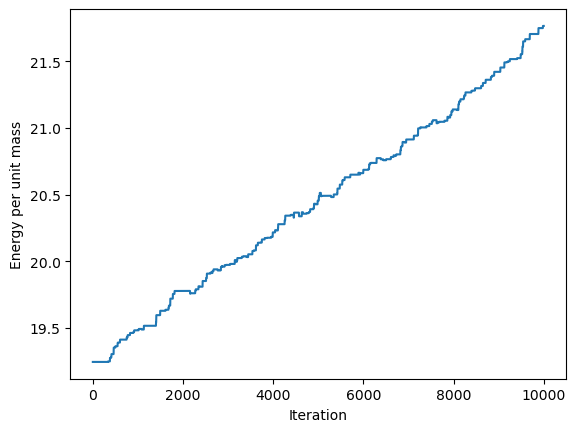

We see that there is an energy variation of about 13% over the course of the simulation. This isn’t great, but is better than e.g. the Euler method.

Making more complex domains

The logic above can be easily generalized to more complex domains, if we can write them as unions of sets.

A particle’s position will, at any moment in time, belong to one or more domains. It escapes the domains once this number reaches zero, in which case we need to know which domain’s boundary was crossed in order to appoint a collision.

This can be done by keeping track of its domain and, once it leaves, use the equations appropriate to this domain to prescribe collision effects.

This doesn’t sound particularly efficient, but we leave this for later.

More precisely, assume we are given $N$ functions $\omega_A$ for domains $\Omega_A$ given by their positive support. At any moment $t$, for a particle at $x_t$, the set

$$I_t = \{A: \omega_A(x_t) > 0\}$$

is non-empty, and counts in which domain(s) the particle is.

Now, consider the wall collision case where $I_{t+1} = \mathrm{empty}$ but $I_t = A$ for some index $A$. Then, we can use the collision conditions for $A$, ie. $\omega_A$, $\nabla \omega_A$ etc. in the same way as above.

As an implementation, we will slightly modify the Particle class to add a method which identifies in which domain it is.

class Particle:
    def __init__(self, x0, v0, label=None, domain=None):
        self.x = x0
        self.v = v0
        self.label = label
        self.domain = domain
    
    def evolve_temp(self, dt, method='leapfrog'):
        self.x_, self.v_ = evolution(self.x, self.v, dt, method=method) 
        return self

    def validate_evolution(self):
        self.x = self.x_
        self.v = self.v_
        return self
    
    def attribute_one_domain(self, omega_func, indices) :
        """
        Given possible domains, find at least one where the particle is

        Inputs:
        omega_func: function receiving (position, index); omega_A(x)
        indices: list of indices to test
        """
        
        for index in indices:
            if omega_func(self.x, index) > 0:
                self.domain = index
                break
                
        return self

# Need three regions
def omega(pos, index):
    x, y = pos

    match index:
        case 1:
            return 1 - (x+2)**2 - y**2
        case 2:
            return 1 - (x-2)**2 - y**2
        case 3:
            return 5 - x**2 - (y+2)**2
        case _:
            raise

def grad_omega(pos, index):
    x, y = pos
    match index:
        case 1:
            return - 2 * np.array([x+2, y])
        case 2:
            return - 2 * np.array([x-2, y])
        case 3:
            return - 2 * np.array([x, y+2])
        case _:
            raise

def hessian(pos, index):
    return -2*np.eye(2)

# new function: finds domain where the particle lives
def current_domain(pos, omega_func, indices):
    for index in indices:
        if omega_func(pos, index) > 0:
            return index
    return None

Now we basically copy-paste the code above:

# Random initial positions
# Initialize 600 particles initially and keep those who fall inside our domain

n_base = 600
np.random.seed(32)
x = np.random.uniform(-4,4, size=n_base)
y = np.random.uniform(-4,1, size=n_base)

survives = [current_domain(np.array([xx,yy]), omega, indices=[1,2,3]) for xx, yy in zip(x, y)]
x = [xx for xx, s in zip(x, survives) if s is not None]
y = [xx for xx, s in zip(y, survives) if s is not None]

initial_positions = np.array([x,y]).T
n = len(initial_positions)
print(n)

311

# new: indices and attribution
indices = [1,2,3]

particles = [Particle(x, np.zeros_like(x), label=i).attribute_one_domain(omega, indices)
             for i, x in enumerate(initial_positions)]

positions = [particle_list_to_scatter(particles)]
speeds = [particle_list_to_speeds(particles)]


for t in tqdm(time_range):
    for part in particles:
        part.evolve_temp(dt)
        new_domain = current_domain(part.x_, omega, indices)
        if new_domain is None: # the particle fell out
            last_index = part.domain
            dx = part.x_ - part.x
            omega_x, domega_x, hessian_x = omega(part.x, last_index), grad_omega(part.x, last_index), hessian(part.x, last_index)
            lamb = - omega_x/ (dx @ domega_x)
            normal = normalize(domega_x + lamb * (hessian_x @ dx))

            # update position
            new_part_x = part.x_ - 2*(1-lamb)*(dx @ normal) * normal

            # update speed
            part.evolve_temp(lamb * dt)
            new_part_v = part.v_
            
            # finalize
            part.v_ = new_part_v - 2*(new_part_v @ normal) * normal
            part.x_ = new_part_x
        elif new_domain != part.domain: # the particle went into a new domain, but is still inside 
            part.domain = new_domain
            
        part.validate_evolution()
    
    positions.append(particle_list_to_scatter(particles))
    speeds.append(particle_list_to_speeds(particles))

Again, we capture the “video” of the particles’ motion:

%%capture
colors = cm.rainbow(np.linspace(0, 1, n))
fig, ax = plt.subplots(figsize=(8,8))
camera = Camera(fig)

ax.set_aspect(1)

for i, aux in enumerate(positions):
    if i % 20 == 0:
        time = time_range[i]
        circ1 = plt.Circle((-2,0), 1, color='LightGray', zorder=1, alpha=0.5)
        circ2 = plt.Circle((2,0),  1, color='LightGray', zorder=2, alpha=0.5)
        circ3 = plt.Circle((0,-2), np.sqrt(5), color='LightGray', zorder=3, alpha=0.5)
        ax.add_artist(circ1)
        ax.add_artist(circ2)
        ax.add_artist(circ3)
        ax.scatter(aux[:,0], aux[:,1], c=colors, zorder=100)
        camera.snap()
    
anim = camera.animate(blit=False, interval=40) #  miliseconds

anim.save('collisions2.gif') # save as gif

HTML(anim.to_jshtml())