Attention: a tale of three spaces

Motivation

I admit I always had some trouble understanding Attention in the context of Transformers.

There are several good references for this - Jay Alammar’s The Illustrated Transformer is a common example. Still, I always had some difficulties building a mental model of what the attention mechanism does. Some references explain very thoroughly how to make the calculation, but not exactly why it works.

Recently, I decided to try and write down an explanation that I can refer to in the future, for when I inevitably forget some details. This post is meant to be such explanation. The fact that these notes are mainly intended for self-reference means that they are highly overfit to my own way of thinking, and may not be as useful for other people with different backgrounds. I leave a list of several good resources in the References section.

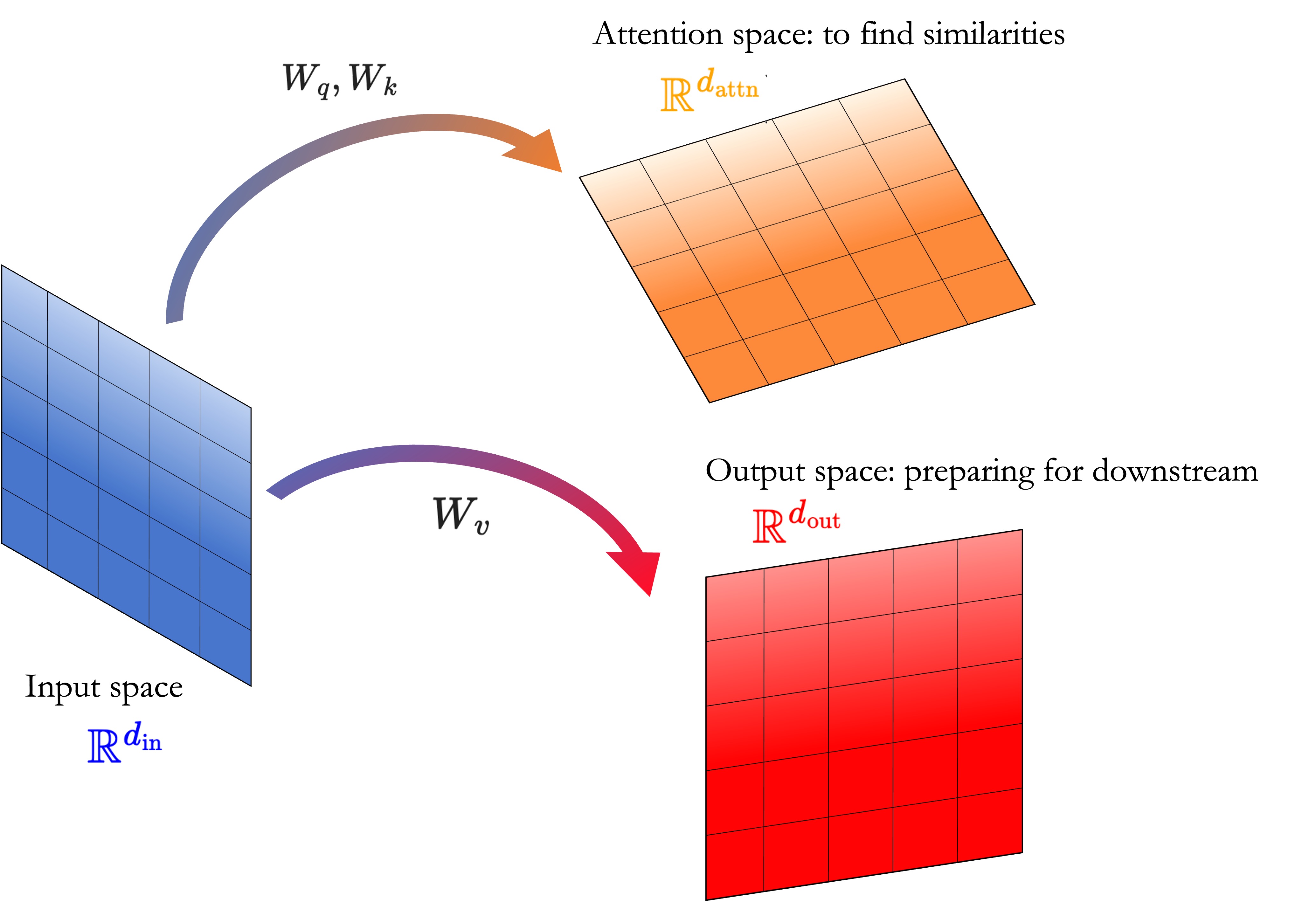
The TL;DR of Attention is that it is a smart way to map embedding vectors (ie. vectors representing words) to an inner product space where similarities among words can be measured; these similarities are then used as weights to create new vectors from the original ones in yet another vector space. Because there are at least three vector spaces appearing here — the original input space; the space where we calculate similarities; and the output space where we build a new vector — I like to think of Attention as an interplay of these 3 spaces.

Notational challenges

The original Transformers paper (Vaswani et al, 2017) employs a convention where:

• $d$-dimensional vectors are row-wise. For example, $x \in \mathbb R^3$ can be written as

  $$x = \begin{bmatrix}1.2 & 2.1 & -0.4 \end{bmatrix} \quad (\text{Transformers paper}),$$

  which differs from the math / physics usual convention of treating them as columns: $x = \begin{bmatrix} 1.2 \\ 2.1 \\-0.4 \end{bmatrix}\quad (\text{Math, Physics})$

• Linear maps act on vectors from the right: if $A: \mathbb R^d \to \mathbb R^d$ is a linear map, its action on a vector $x$ is computed as the matrix product $xA$. For the vector above, if we consider

  $$A = \begin{bmatrix} 2 & 0 & -1 \\ -1 & 3 & 0 \\ 1 & 1 & 1\end{bmatrix},$$

  then

  $$x A = \begin{bmatrix}1.2 & 2.1 & -0.4 \end{bmatrix} \begin{bmatrix} 2 & 0 & -1 \\ -1 & 3 & 0 \\ 1 & 1 & 1\end{bmatrix}= \begin{bmatrix} -0.1 & 5.9 & -1.6 \\\end{bmatrix}.$$

To make sense of things, I can’t help but transpose this notation to a more traditional one where vectors are columns and linear maps happen from left: $x \mapsto A x$. This is also what Phuong, Hutter (2022) do in their notes.

Finally, in what follows, I use $\mathrm{Mat}(n\times m)$ to denote real matrices with $n$ rows and $m$ columns; I find this a bit easier to read than the more common notation $\mathbb R^{n\times m}$. It is clearly inspired by a great teacher I’ve had.

The basic goal of attention is to “stretch and rotate” word embeddings given their contexts

The goal of attention (and, more specifically, self-attention) is to be a layer that helps a neural network look at other words in the input sentence as it encodes a specific word. It provides a way to convert a word and its context into a useful vector representation, to be sent downstream into the neural network.

This paragraph was paraphrased from The Illustrated Transformer.

In other words, attention is a map taking an input token and its context into a vector representation of the context which is useful for deep learning applications.

Overview of the Attention logic

We adapt Algorithm 3 in Phuong, Hutter (2022), describing attention for a single token as a means to make the mechanism clearer. We deal with the computationally optimized version afterwards.

Consider a sentence $\mathbf x = [x_1 \; x_2 \; \ldots \; x_T]$ with $T$ tokens. For example, “I like apples” has $T=3$ tokens $x_1 = \text{I}$, $x_2 = \text{like}$ and $x_3 = \text{apples}$.

We will assume an initial embedding layer / function is defined, taking tokens to some vector representation in $d_\mathrm{in}$ dimensions. This construction can be as simple as a lookup table for a one-hot encoded vocabulary: see Algorithms 1 and 2 of Phuong, Hutter (2022).

Now, we consider the attention calculation for a given token $x$ and its context $(x_t)_{t=1}^T$ . It is divided in two-parts:

• Similarity calculation: we “compare” the current token with the others via a properly-chosen operation, namely, an inner product;
• Value calculation: we construct a linear combination of all context vectors, weighted by their similarities to the current token. The resulting vector is a proper weighted sum of all context vectors considering how much “attention” each word gives to the chosen token.

The whole process consists of properly constructing linear transformations that “optimize” the similarity calculations, and then constructing a new embedding that combines all the information into a single vector.

Scaled dot-product: a smart way to compute similarities

In machine learning, one often considers vector spaces where lengths of vectors don’t matter as much as the angle between any two of them (what one calls in a projective vector space in mathematics - physicists are used to this construction from Hilbert spaces, where vectors must be projected to the unit sphere).

In a world where vectors are normalized to 1, the “similarity” between two vectors $\vec a$, $\vec b$ can be naturally defined from the so-called “cosine similarity”

$$\cos \theta := \vec a \cdot \vec b,\quad \text{since} \quad \|\vec a\|=\|\vec b\|=1.$$

Cosines closer to 1 = high similarity; closer to -1 = low similarity.

Inner products are not uniquely defined, though, and we can make use of that (indeed if $\langle \cdot , \cdot \rangle$ is an inner product then $\langle \cdot, M \cdot \rangle$ is also an inner product, where $M$ is a positive-definite symmetric matrix). We will define a new inner product in $\mathbb R^d$, the so-called scaled-dot product, which is suitable for high dimensions. Let

$$\langle \vec a, \vec b \rangle:=\frac{\vec a \cdot \vec b}{\sqrt{d}}=\frac{1}{\sqrt{d}}\sum_{i=1}^d a_i b_i.$$

It is easy to show that this operation satisfies all properties of an inner product, so it is a valid definition.

Why do we define it this way? As Vaswani et al, 2017 argue, it is because it works: it brings the inner products to numerically treatable values that do not saturate downstream functions.

One can ad-hoc justify this choice of scaling the standard dot product by the means of an example: let $X_i, Y_i \sim \mathrm{Uniform}([-a,a])$, for some $a>0$, be the iid. components of two $d$-dimensional random variables. It is easy to show that $\mathbb E[\vec X\cdot \vec Y] = 0$ and $\mathrm{Var}[\vec X \cdot \vec Y]=Cd$ with $C$ being constant. Notice how the spread grows linearly with the dimension $d$. Now, using the scaled-dot inner product yields $\mathbb E\langle \vec X, \vec Y\rangle=0$ and $\mathrm{Var}\langle\vec X,\vec Y\rangle=C$ which is a constant that doesn’t depend on $d$. Therefore, this scaling helps us keep things within the same order of magnitude.

For all that matters, we don’t need to think about this scaling too much; simply consider it as our default inner product.

The three vector spaces

We have three spaces which are relevant here:

• Input space, with dimension $\color{blue}{d_\mathrm{in}}$: where our embeddings live;
• Attention space, with dimension $\color{orange}{d_\mathrm{attn}}$, where dot products are calculated: it is meant to be the “best” space for computing similarities;
• Output space with dimension $\color{red}{d_\mathrm{out}}$: these are the vectors that will be sent to fully connected layers downstream. It is meant to be the “best” space to encode the vectors for the specific application of the model (eg: next-token prediction.)

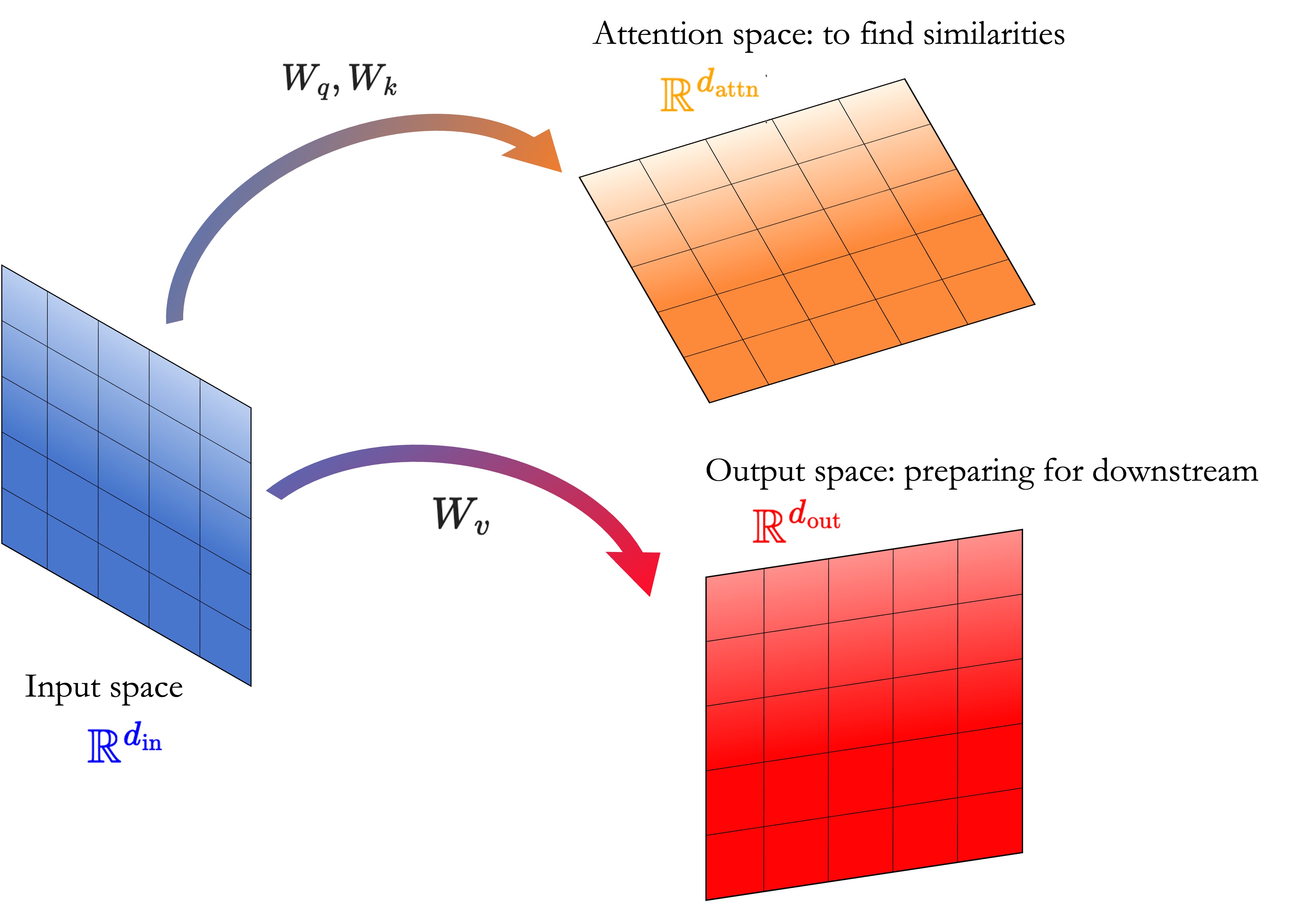
The whole point of attention is to construct linear transformations taking embeddings to new vector spaces where similarities are more explicit. Now, linear transformations between vector spaces are naturally defined in terms of matrices, so these will appear as trainable parameters $W_k, W_q$ and $W_v$ (plus biases) as we will see below.

Note: the letters $Q$, $K$ and $V$, used above and below, refer to “queries”, “keys” and “values”, which evoque the analogous terms in database theory. I don’t love these names, but they are now so deeply rooted in the literature that we have no option but to get used to them.

The logic behind them is that we compare a specific token (our “query”) to all other tokens in the context (the “keys”); those context words which are very similar to the query gain a high “value”.

With this preamble done, let’s dive into the algorithm:

Attention algorithm

Inputs:

• $e \in \color{blue}{\mathbb R}^{\color{blue}{d_\mathrm{in}}}$: the embedding of the current token being considered;
• $e_t \in \color{blue}{\mathbb R}^{\color{blue}{d_\mathrm{in}}},\quad t = 1,\ldots, T$: the embeddings of the tokens in the current token’s context (for self-attention, it can be the words in the sentence the current token belongs to).

Obs #1: Notice that the context may or may not contain the current token itself - it will contain it in cases such as self-attention where we compare a sentence to itself, but it may not in cases such as cross-attention in a sequence-to-sequence task.

Obs #2: we assume context and query embeddings have the same dimensions $d_\mathrm{in}$. This is OK, but we could also allow them to have different dimensions — see parallel attention calculation below.

Trainable parameters:

• $W_q, W_k \in \mathrm{Mat}(\color{orange}{d_\mathrm{attn}} \times \color{blue}{d_\mathrm{in}})$: “query” and “key” matrices, taking vectors from the Input space to the Attention space;
• $W_v \in \mathrm{Mat}(\color{red}{d_\mathrm{out}} \times \color{blue}{d_\mathrm{in}})$: “value” matrix, taking vectors from the Input space to the Output space;
• Bias vectors $b_k, b_q \in \color{orange}{\mathbb R}^{\color{orange}{d_\mathrm{attn}}}$ and $b_v \in \color{red}{\mathbb R}^{\color{red}{d_\mathrm{out}}}$.

Output:

• $\tilde v \in \color{red}{\mathbb R}^{\color{red}{d_\mathrm{out}}}$: vector returning the “total weighted value” of the context of the current token.

Algorithm:

1. First, we map the embedding of the current token onto Attention space via the “query” linear operator (plus a bias term):

   $$q = W_q e + b_q\quad (\in \color{orange}{\mathbb R}^{\color{orange}{d_\mathrm{attn}}})\tag{query projection}$$

2. We do the same for all context tokens, through the “keys” linear operator (plus a bias term):

   $$k_t = W_k e_t + b_k,\quad \forall t \in \{1,\ldots,T\}\quad (\in \color{orange}{\mathbb R}^{\color{orange}{d_\mathrm{attn}}})\tag{key projection}$$

3. We compute the similarity scores between these vectors in Attention space, via the scaled-dot product:

   $$s_{qt} \equiv \langle q, k_t\rangle=\frac{q\cdot k_t}{\sqrt{\color{orange}{d_\mathrm{attn}}}}\tag{similarity calculation}$$

4. We create weights $\alpha_t$ for each context vector; these are positive, normalized, and such that highly similar vectors (ie. those whose inner product is high) get boosted while highly dissimilar vectors (ie. those with very negative inner product) get very small weights:

   $$\alpha_t = \frac{\exp s_{qt}}{\sum_u \exp s_{qu}} =: \mathrm{soft}\max_u(s_{qu})\tag{similarity normalization}$$

   such that $\sum_t \alpha_t = 1$. Any positive, smooth, monotonically increasing function $\phi$ would work here; we could have chosen $\phi(s_{qt})/\sum_u \phi(s_{qu})$ instead of the softmax and everything would work fine.

5. We are ready to compute the output vector. For that, first, map the original context tokens onto the output space via the “values” matrix (plus a bias term), making them almost ready to send forward…

   $$v_t = W_v e_t+b_v,\quad \forall t \in \{1,\ldots,T\}\quad (\in \color{red}{\mathbb R}^{\color{red}{d_\mathrm{out}}}) \tag{value projection}$$

6. … and then compute their weighted sum based on the attention weights:

   $$\tilde v = \sum_t \alpha_t v_t.\tag{output computation} \quad (\in \color{red}{\mathbb R}^{\color{red}{d_\mathrm{out}}})$$

7. Return $\tilde v$.

That’s it.

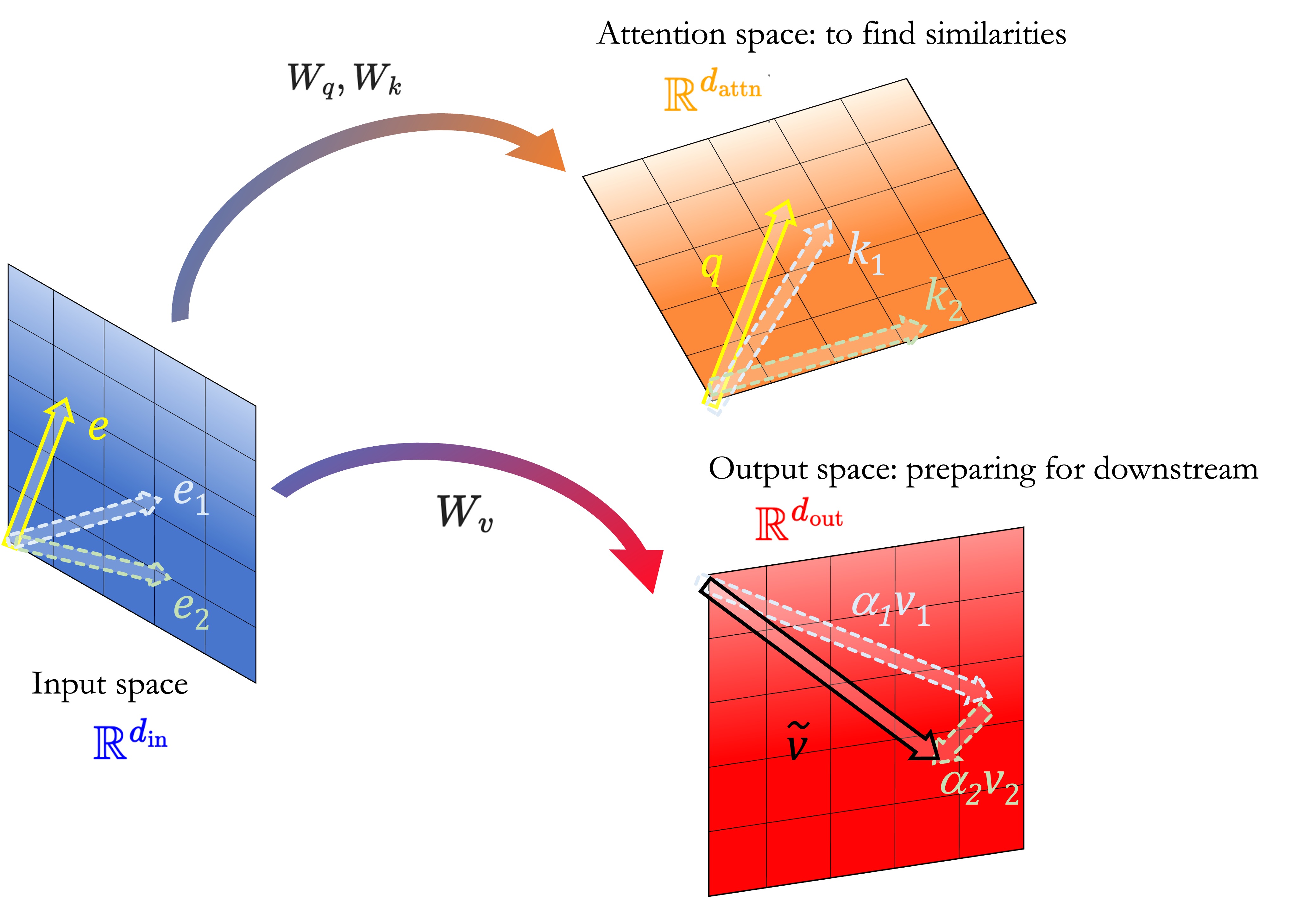
In the cartoon above, we illustrate the Attention mechanism for a context with two key vectors $\color{blue}{e_1}$ and $\color{green}{e_2}$ and a query vector $\color{orange}{e}$, living in the Input space:

• We set all bias vectors to zero for simplicity;
• By mapping the query and key vectors to Attention space, we see that the key $\color{blue}{k_1} = W_k \color{blue}{e_1}$ is close to the query $\color{orange}{q} = W_q \color{orange}{e}$ and thus will get a big weight $\color{blue}{\alpha_1}$ associated to it;
• In contrast, the key $\color{green}{k_2}$ is almost perpendicular to $\color{orange}{q}$ and will have a small weight $\color{green}{\alpha_2}$ associated to it.
• We store these values and create, in the output space, the final vector $\tilde v = \color{blue}{\alpha_1 v_1} + \color{green}{\alpha_2 v_2}$ where each $v_i$ comes from applying the $W_v$ matrix to the context embeddings $\color{blue}{e_1}$ and $\color{green}{e_2}$.

Thinking in terms of (rough) projections

Recall that, in linear algebra, we can construct the projection of a vector $u$ onto a subspace $S$ spanned by an orthonormal basis $\{v_i\}$ as

$$\mathrm{proj}_S \;u = \sum_i \langle v_i, u\rangle v_i$$

This is, in spirit, similar to what attention is doing. To see this, let’s go full hand-wavy and:

• Ignore the exponentials used in softmax; pretend we just want to use $\langle q, k_t\rangle$ instead of its $\exp$;
• Assume all dimensions are the same, ie. $\color{blue}{d_\mathrm{in}} = \color{red}{d_\mathrm{out}} = \color{orange}{d_\mathrm{attn}}$;
• Assume all matrices $W_q, W_k$ and $W_v$ are equal to some matrix $W$. Then, in particular, $k_t = v_t.$

Then, the output computation can be written as

$$v = \sum_t \alpha_t v_t \propto\sum_t \langle k_t, q \rangle k_t.$$

Now, the expression on the right-hand side is not a projection since the $k_t$ are not, generally, orthogonal, nor normalized to 1. I like to think of this expression as a “rough” projection: it is a vector in the space spanned by the $k_t$‘s, but it double-counts projections which are linearly dependent of each other, and it gets the scale completely wrong since we are not normalizing anything.

How things go from here

Once the vector $\tilde v$ is obtained, it is very common across the Transformer-based algorithms to add it back to the original query embedding, hence

$$e \mapsto e + \tilde v$$

(this is often accompanied by a Dropout operation). This is done outside the Attention step, but I like to think of this step as really being the one who finishes the Attention calculation. If we add a “time” index $\tau$ to our vectors, such that before Attention we are at “time” $\tau$ and after Attention we are at time $\tau+\Delta \tau$, then one can write, from the considerations above,

$$\boxed{e_{\tau+\Delta \tau} = e_\tau + \mathrm{Attention}(e_\tau, W\text{'s}).}$$

This feels like a skip connection, and physicists among you will be itching to somehow take $\Delta \tau \to 0$ and make this into a differential equation; indeed, this is exactly what a few papers do, see this and this reference by Geshkovski and collaborators.

Parallelizing Attention

Finally, we comment a bit on the computational side of things.

The great strength of Attention compared to previous RNN-based approaches is that it can be parallelized, and this is how the algorithm is usually presented. Since we have already gained intuition about the process for a single query vector, we can now generalize to parallel computations.

Below, we present a simplified version of Algorithm 4 of Phuong, Hutter (2022) in the case of unmasked attention. We allow query vectors and context embedding vectors to have possibly different dimensions; then, we have indeed two “Input” spaces compared to a single one as we had above.

Also, we drop the colors on the different spaces :)

Inputs:

• $X \in \mathrm{Mat}(d_X \times L_X)$: a matrix where each of its $L_X$ columns is the embedding vector of a token, itself a vector in $\mathbb R^{d_X}$;
• $Z \in \mathrm{Mat}(d_Z \times L_Z)$: a matrix where each of its $L_Z$ columns is a context vector, each a vector in $\mathbb R^{d_Z}$.

Trainable parameters

• $W_q \in \mathrm{Mat}(d_\mathrm{attn} \times d_X)$: maps query vectors to Attention space
• $W_k \in \mathrm{Mat}(d_\mathrm{attn} \times d_Z)$: maps key vectors to Attention space
• $W_v \in \mathrm{Mat}(d_\mathrm{out} \times d_Z)$: maps key vectors to the Output space
• $b_q, b_k \in \mathbb R^{d_\mathrm{attn}}, b_v \in \mathbb R^{d_\mathrm{out}}$: bias terms

Outputs:

• $\tilde V \in \mathrm{Mat}(d_\mathrm{out} \times L_Z)$: matrix containing total weighted values of all context tokens considered.

Algorithm:

• As before, we map query embeddings to Attention space via

  $$Q = W_q X+ b_q\mathbf 1 \quad (\in \mathrm{Mat}(d_\mathrm{attn}\times L_X))$$

  where $\mathbf 1$ is a column vector with all elements equal to 1.

• Similarly, we map key embeddings to Attention space via

  $$K = W_kZ+b_k\mathbf 1\quad (\in \mathrm{Mat}(d_\mathrm{attn}\times L_Z))$$

• We compute similarity scores as

  $$\alpha=\mathrm{softmax}\left(\frac{K^T Q}{\sqrt{d_\mathrm{attn}}}\right) \quad (\in \mathrm{Mat}(L_Z\times L_X))$$

  with the override of the softmax functions to matrices in $\mathrm{Mat}(L_z \times L_X)$ defined component-wise as

  $$\mathrm{softmax}(A)_{z,x}:= \frac{\exp A_{z,x}}{\sum_{z'} \exp A_{z',x}}.$$

• To obtain the output, we need to first map all key vectors to the Output space, via

  $$V=W_vZ+b_v \mathbf 1 \quad (\in \mathrm{Mat}(d_\mathrm{out}\times L_Z))$$

  and then act on them with the weights:

  $$\tilde V = V \alpha = V \;\mathrm{softmax}\left(\frac{K^T Q}{\sqrt{d_\mathrm{attn}}}\right) \quad (\in \mathrm{Mat}(d_\mathrm{out} \times L_Z)).$$

  Hence, we get a final matrix which contains the output vector for all context vectors. This last formula is, in our notation, the first equation in the classic Transformers paper (Vaswani et al, 2017).

References

[1] These two videos are great, and explain Attention very intuitively from the point of view of linear transformations: Video 1: link Video 2: link

[2] Mary Phuong and Marcus Hutter, Formal Algorithms for Transformers, DeepMind, 2022. This was the main reference for the pseudocode here.

[3] The 2023 Stanford XCS224U Natural Language Understanding lecture on Attention is perhaps the best class I’ve ever seen on the topic, mixing theory, diagrams and code. In fact, the whole playlist is a gem worth watching and rewatching.

[4] A surprisingly good explanation in Wikipedia

[5] The Annotated Transformer. A walkthrough of Attention paper with code: https://nlp.seas.harvard.edu/2018/04/03/attention.html

[6] Jay Allamer’s The Illustrated Transformer

[7] Of course, the original Transformers paper by Vaswani et al (2017) - although I tend to find it rather hard to understand.